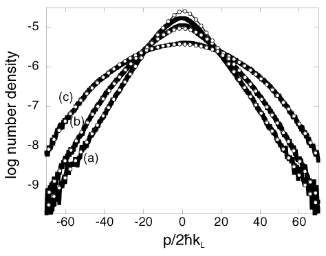
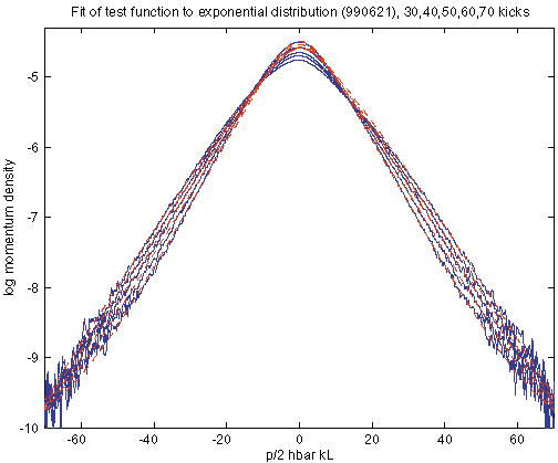
| Exponential localization: | g = 1.06 ± 0.19, b = 0.06 ± 0.17 |
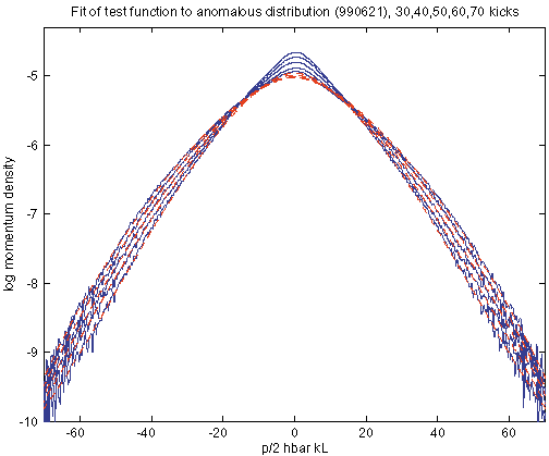
| Regime of classical anomalous diffusion: | g = 1.48 ± 0.16, b = 0.32 ± 0.07 |
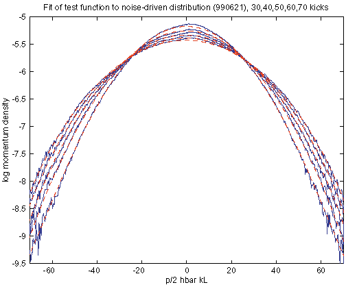
| Noise-induced delocalization: | g = 2.03 ± 0.14, b = 0.51 ± 0.03 |
Text to be included in the paper is posted here as a
LaTeX file (plain text),
and in compiled form as
postscript and
pdf.
The revised composite plot (to appear in the paper) for the three cases showing the experimental data with the fits at 70 kicks in .eps format is posted here (old one is here), and this is what it looks like:

The raw data used to make the above plot is posted here also; the format here is 6 columns per file, the first column being the momentum axis and the others are the distributions for 30, 40, 50, 60, and 70 kicks (in zip (pc) or sit.hqx (mac) format.
The fits are performed simultaneously on the measured distributions at 30, 40, 50, 60, and 70 kicks. We also have measurements at 0, 10, and 20 kicks, but they are excluded from the fit in order to focus on long-time effects. The distribution used for the fit is
F(p) = A exp(-|(p-p0)/w|g),
where g is a fitting parameter common to all the distributions in the fit, A is the amplitude factor, and p0 the center offset. The width parameter w is constrained to satisfy
w(t) = w0 + a tb,
where w0 and a are fitting parameters, and b is given by 1 - 1/g. In the fit, each distribution is convolved with the initial distribution and then corrected for the known response of the detection system (i.e., the nonuniformity of the Gaussian imaging laser beams).
After convolution and detection system correction, the distributions are corrected for baseline offsets that may be introduced in the experimental measurement, by adding a constant f to each distribution, according to f(t) = f0 + f1 t, where f0 and f1 are fitting parameters. This linear model for the baseline offsets is justified by fits where the baseline offsets at each time are treated as five independent parameters. Similarly, the amplitudes A for the distributions are constrained to satisfy A(t) = A0 + A1 t + A2 t2, where A0, A1, and A2 are fitting parameters. This constraint is likewise justified from fits where the five amplitudes are independent parameters. These constraints on f and A are important in making the fitting results stable against changing the cutoff locations, as described below. The center offsets p0 are treated as five independent parameters, since they are well decoupled from the other parameters. It is necessary to include these offsets to account for possible drifts of the atomic cloud from shot to shot.
In order to emphasize the tails of the distribution during the fit, the logarithm of the data is taken before it is sent to the Marquardt-Levenberg fitting routine. Additionally, the data near the center is excluded, along with the data in the extreme tails of the distributions where the signal-to-noise ratio is bad. These “cutoff values” are varied in order to gauge the sensitivity of the fit to this procedure; the dominant error in the fitting exponent comes from variations in the exponent due to different cutoffs, which seems to indicate that data at longer times and with better signal/noise ratios would give more precise numbers. All the data are weighted equally, using the mean uncertainty for each data point in order to get a meaningful value of the c2 statistic. As discussed below, the uncertainties returned by the fitting routine are on the order of a few percent, which is much smaller than the final uncertainties that we quote.
The primary contribution to the fitting uncertainty in g is the sensitivity to the exact locations of the data exclusion boundaries. The summary of the fit results below lists the boundaries as “clip xx, yy:”, where the data with |p| < xx or |p| > yy (with p in units of double photon recoils) are excluded. The boundary set (15, 70) is used as the final and representative value in the three cases, and the other values are used to set the fitting uncertainty (which is larger than that reported by the Marquardt-Levenberg fitting algorithm for a single fit). The other numbers reported in the summary are the c2 statistic, along with c2 divided by the number of degrees of freedom, which should be close to 1 for a good fit.
For the values of g listed here, the values seem to cluster near 1.06 or 1.25. The values near 1.25 are associated with an outer boundary of 60, and the tails beyond 60 diverge too quickly from the data. Hence, the value of 1.06 is probably the more reliable candidate, and we quote a relatively large uncertainty of ±0.19 in order to account for the possibility of a larger exponent, based on the numbers here and experience with other variants on the model described above.
|
Summary of Fit Results: clip 15, 60: gamma = 1.27, chisq = 2427, chisq/ndeg = 1.825 clip 20, 60: gamma = 1.25, chisq = 1956, chisq/ndeg = 1.656 clip 25, 60: gamma = 1.27, chisq = 1608, chisq/ndeg = 1.554 clip 15, 65: gamma = 1.14, chisq = 2295, chisq/ndeg = 1.551 clip 15, 70: gamma = 1.06, chisq = 2504, chisq/ndeg = 1.541 <--- clip 20, 70: gamma = 1.06, chisq = 2213, chisq/ndeg = 1.496 clip 25, 70: gamma = 1.05, chisq = 1943, chisq/ndeg = 1.461 clip 15, 75: gamma = 1.06, chisq = 2314, chisq/ndeg = 1.304 clip 20, 75: gamma = 1.05, chisq = 2095, chisq/ndeg = 1.286 clip 25, 75: gamma = 1.04, chisq = 1881, chisq/ndeg = 1.271 clip 15, 80: gamma = 1.04, chisq = 4192, chisq/ndeg = 2.184 |
The exponent values here lie in the range from 1.4 to 1.6, with one outlier at 1.75. The fits seem to be most reliable if not too much of the center is excluded, so the outlier can probably be ignored. Still, in order to account for a possibly smaller exponent seen in other versions of the fitting model, we quote g = 1.48 ± 0.16.
|
Summary of Fit Results: clip 15, 60: gamma = 1.47, chisq = 2476, chisq/ndeg = 1.862 clip 20, 60: gamma = 1.61, chisq = 1994, chisq/ndeg = 1.688 clip 25, 60: gamma = 1.75, chisq = 1603, chisq/ndeg = 1.549 clip 15, 65: gamma = 1.54, chisq = 2430, chisq/ndeg = 1.648 clip 10, 70: gamma = 1.43, chisq = 1828, chisq/ndeg = 1.030 clip 15, 70: gamma = 1.48, chisq = 1628, chisq/ndeg = 1.002 <--- clip 20, 70: gamma = 1.54, chisq = 1451, chisq/ndeg = 0.981 clip 25, 70: gamma = 1.61, chisq = 1289, chisq/ndeg = 0.970 clip 30, 70: gamma = 1.52, chisq = 1133, chisq/ndeg = 0.961 clip 15, 75: gamma = 1.45, chisq = 2574, chisq/ndeg = 1.450 clip 20, 75: gamma = 1.48, chisq = 2356, chisq/ndeg = 1.445 clip 25, 75: gamma = 1.48, chisq = 2136, chisq/ndeg = 1.443 |
The fitted exponents in this case generally range between 1.9 and 2.1, with one notable outlier at 2.20. This outlier points to an unreliable fit if too much of the center is excluded from the fit, so that “momentum boundary” effects artificially raise the exponent value (because the boundary effects cause steeper tails in the distribution due to reduced transport). The exponents are otherwise consistent with the expected value of 2.0 for normal diffusion, so for this case we quote g = 2.03 ± 0.14.
|
Summary of Fit Results: clip 10, 60: gamma = 1.89, chisq = 711, chisq/ndeg = 0.480 clip 15, 60: gamma = 1.90, chisq = 622, chisq/ndeg = 0.468 clip 20, 60: gamma = 1.96, chisq = 522, chisq/ndeg = 0.442 clip 10, 70: gamma = 2.01, chisq = 1058, chisq/ndeg = 0.596 clip 15, 70: gamma = 2.03, chisq = 959, chisq/ndeg = 0.590 <--- clip 20, 70: gamma = 2.09, chisq = 858, chisq/ndeg = 0.581 clip 25, 70: gamma = 2.20, chisq = 756, chisq/ndeg = 0.569 clip 20, 75: gamma = 2.01, chisq = 1204, chisq/ndeg = 0.741 |
